CAIA® return distributions: what do the four moments miss?

On this page

A return distribution is a map of possible returns and how much weight each outcome receives. Its mean, variance, skewness and kurtosis describe location, spread, asymmetry and tail weight, but those summaries cannot establish the probability of a particular future loss. For CAIA® Level I, learn to read the shape, then ask whether the observations and assumptions behind it fit the decision.

Start with the question the distribution answers

An ex post distribution organises returns that have already occurred. An ex ante distribution assigns probabilities to returns that might occur. Confusing the two turns a description of a sample into a forecast. A manager may show many quiet monthly returns; that record tells you what was observed over those months, not how often a large loss must occur next year. A sensible interpretation asks how the sample was selected, whether valuations were timely, and whether the strategy or market setting changed during the period. These questions matter especially when a return series contains infrequently priced assets.

The CAIA curriculum overview places statistical foundations within Level I Introduction to Alternative Investments. The CAIA study tools page directs candidates to the current curriculum companion and stresses that editions are tied to the exam year. Use that companion to check the relevant learning objective, while treating a worked set of invented returns as a method demonstration rather than evidence about a real fund. The skill being tested is interpretation: identify which feature of the distribution answers the stated question, and which feature has not been measured.

Read the centre and spread before the tails

The mean is the probability-weighted centre for a prospective distribution, or the arithmetic average for equally weighted observations. It answers what return is expected under the assigned probabilities. Variance takes each outcome's distance from that mean, squares it, and averages using the same weights. Squaring makes a large miss count more than a small one and prevents gains and losses from cancelling. Standard deviation is the square root of variance, expressed in return units, so it is easier to compare with the original returns. These measures describe different aspects: a high mean does not imply a narrow distribution, and a narrow distribution does not imply attractive outcomes.

Keep the denominator straight. If a question gives an entire probability model, weight each possible outcome by its probability. If it gives a historical sample and asks for a sample variance, the familiar sample correction uses one fewer degree of freedom than the observation count. Do not import that correction into an ex ante scenario table. Nor should you treat a calculated mean as a promise: a discrete distribution can have a mean that is not itself one of the possible returns. The CFA Institute statistical measures reading also distinguishes central tendency, dispersion and shape as separate interpretation tasks.

A small scenario shows what each summary adds

Consider an entirely illustrative private asset strategy with four possible one-period returns. Give a loss of twenty percent a probability of one tenth, a zero return a probability of two tenths, a gain of ten percent a probability of five tenths, and a gain of twenty percent a probability of two tenths. The probabilities sum to one. The weighted mean is a gain of seven percent: the loss contributes minus two percentage points, the zero contributes nothing, and the two gains contribute five and four percentage points. This is an expectation under the invented probabilities, not a realised or predicted market return.

To see the spread, subtract seven percentage points from each possible return. The deviations are minus twenty-seven, minus seven, plus three and plus thirteen points. Square these deviations, weight them by the scenario probabilities, and add them. In squared percentage-point units, the pieces are 72.9, 9.8, 4.5 and 33.8, giving a variance of 121. The standard deviation is therefore eleven percentage points. The mean and standard deviation alone might sound fairly reassuring, yet the table still explicitly assigns a one-in-ten chance to a loss of twenty percent. The invented table, rather than a bell-curve shortcut, supplies that probability.

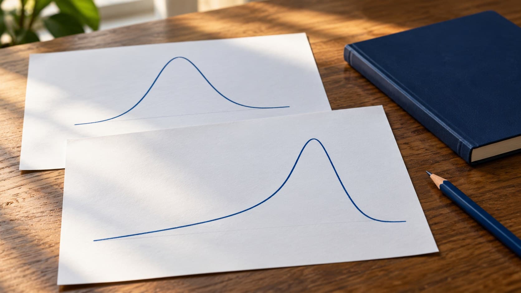
Now look at direction. The large negative deviation lies farther from the mean than the positive deviations, so cubing deviations gives the loss scenario disproportionate negative influence. The distribution has negative skew under these assumed weights. That tells you the long side of its asymmetry points towards losses. It does not mean every observation must be a loss, nor does it tell you the probability of crossing a particular loss threshold without examining the distribution itself. In this example, a candidate who reports only the seven-percent mean misses the event that may dominate the investor's practical concern.

Kurtosis looks at fourth-power deviations after standardising for scale. It is commonly discussed as tail weight relative to a normal benchmark; excess kurtosis subtracts the normal benchmark from the kurtosis measure. A higher value can flag more mass in unusual outcomes than a comparable normal model, but it does not identify which tail creates that mass. The scenario's negative skew already directs attention to the loss side. Avoid calling kurtosis a measure of downside alone: a very large positive outcome can also raise a fourth-power statistic. For an exam answer, state separately what skewness and kurtosis contribute.

Why the normal shortcut can mislead

A normal distribution is symmetric, so its mean and standard deviation define its shape. That is useful for a calculation that explicitly assumes normality. It is a poor silent default when the observed or assumed distribution has an elongated loss tail. If two strategies have similar means and variances, they can still differ in the pattern of rare gains and losses. Treat a normal model as a specified modelling choice, and check whether the task asks for a normal probability or for interpretation of actual scenario weights. Never substitute a normal tail probability for the probability printed in a scenario table.

A lognormal model answers a related but different question. If a log return is modelled as normal, its corresponding positive price relative is lognormal. The price relative cannot be negative, whereas an unconstrained normal price model could imply an impossible negative price. That modelling convenience does not prove that real prices follow a lognormal law or that their tail risk has been fully captured. A question may switch between simple returns, log returns and price levels; check which variable the distribution describes before choosing an interpretation. The same word, return, can hide a different aggregation rule across periods.

The time horizon matters too. A monthly distribution cannot be read as an annual distribution by simply relabelling the axis. Compounding changes simple returns across periods, and dependence between successive outcomes changes the distribution of a long-horizon total. A small monthly sample may contain no severe event because severe events were absent during observation, not because the chance is zero. If a manager changed leverage, asset mix or valuation practice, observations from before the change may poorly represent the new exposure. These are reasons to inspect the assumptions, not invitations to invent a numerical adjustment.

Use the four moments as a diagnostic order

First, identify whether the data are historical observations or assigned future scenarios. Next, find the centre and spread using the weights the question actually supplies. Then read skewness for direction of asymmetry and kurtosis for the relative prominence of unusual outcomes. Finally, return to the investor's decision: is the concern about an average result, variability around that average, a large loss, or a specific threshold? A moment is useful only when it answers that concern. For threshold risk, a scenario table or a separately supported probability model often communicates more than four summary numbers.

When revising, try to explain the invented example without reciting labels. Say why the loss can coexist with a positive mean, why squaring deviations hides their sign, why cubing retains it, and why fourth powers highlight distance rather than direction. Those four explanations expose the usual mistakes more quickly than memorising a row of definitions. The CAIA program page provides the broader study context, and the methodology page explains how to use structured practice alongside the official curriculum. The examination task is to choose the relevant measure and state its limit, not to infer a future tail from a neat historical average.